6 Appendix A — Supplementary Material for “Colour Blinded by the Noise”

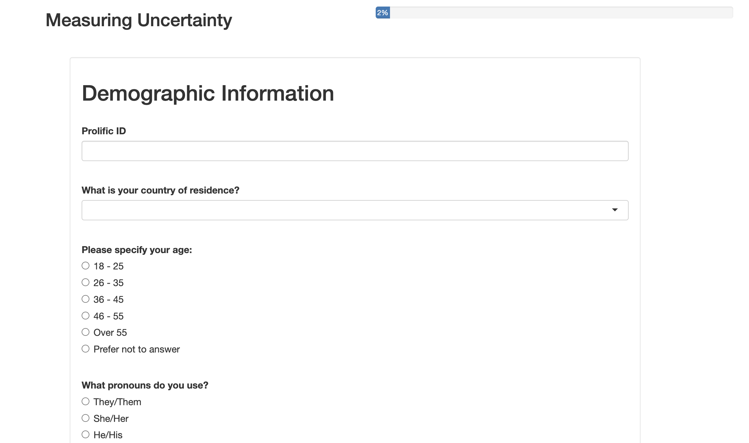
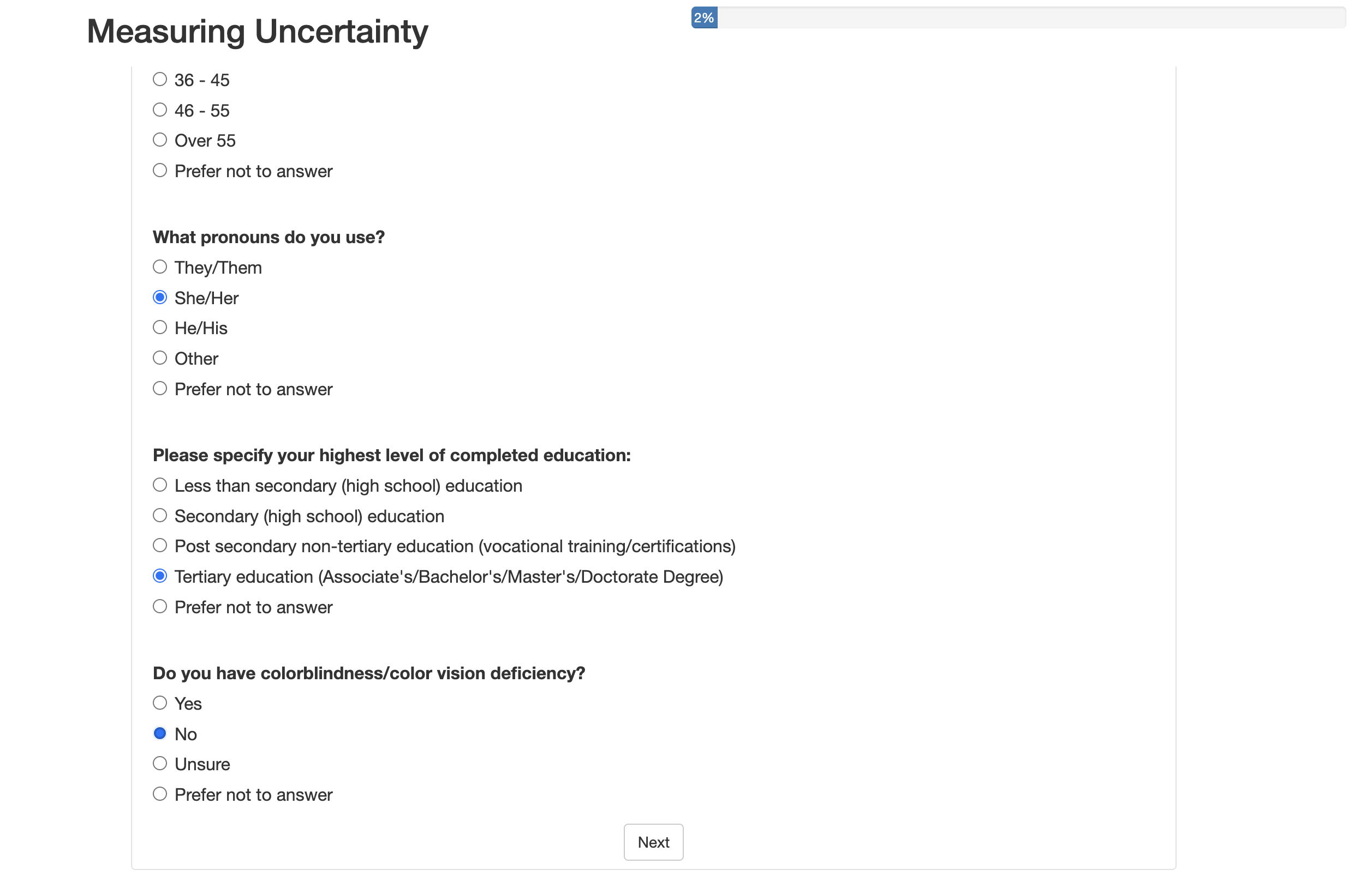
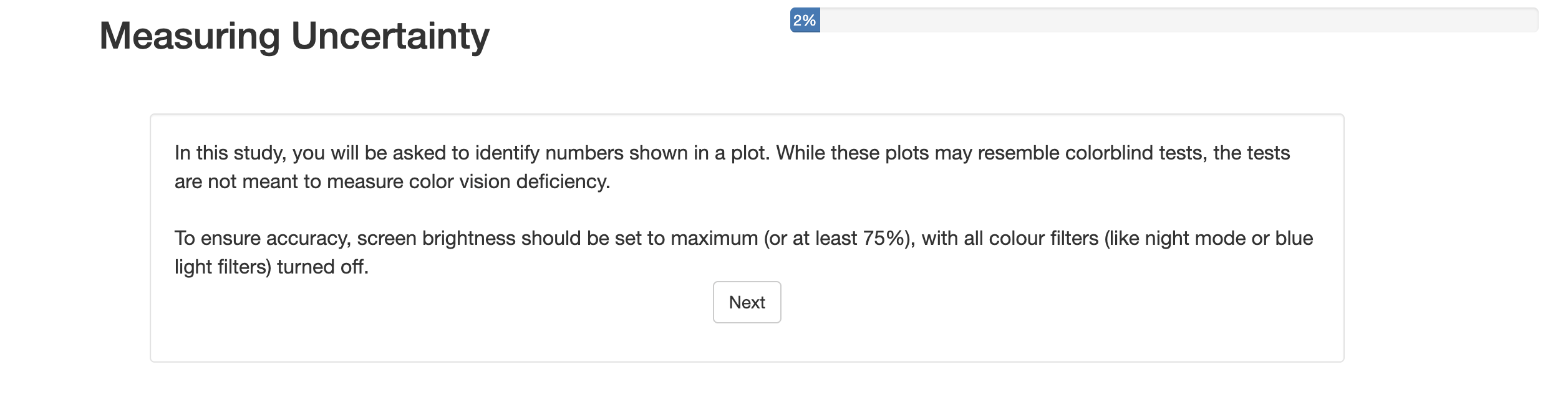
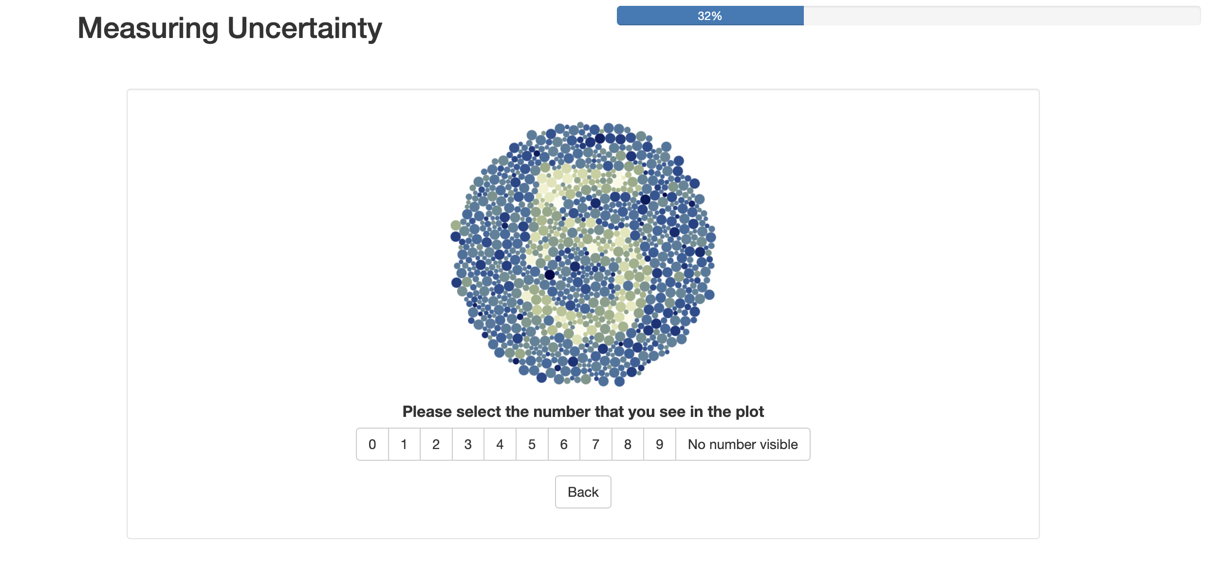
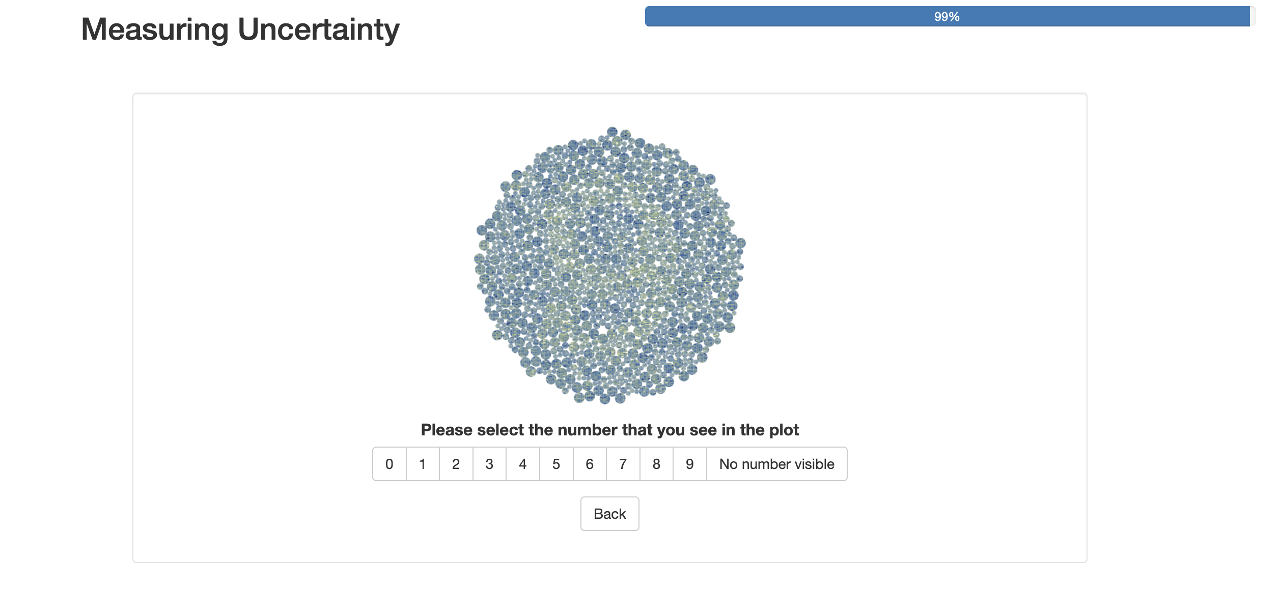
6.1 Full app screenshots

Screenshots from the app, in the order that the participants would experience them.

6.2 Confusion matrix of numbers

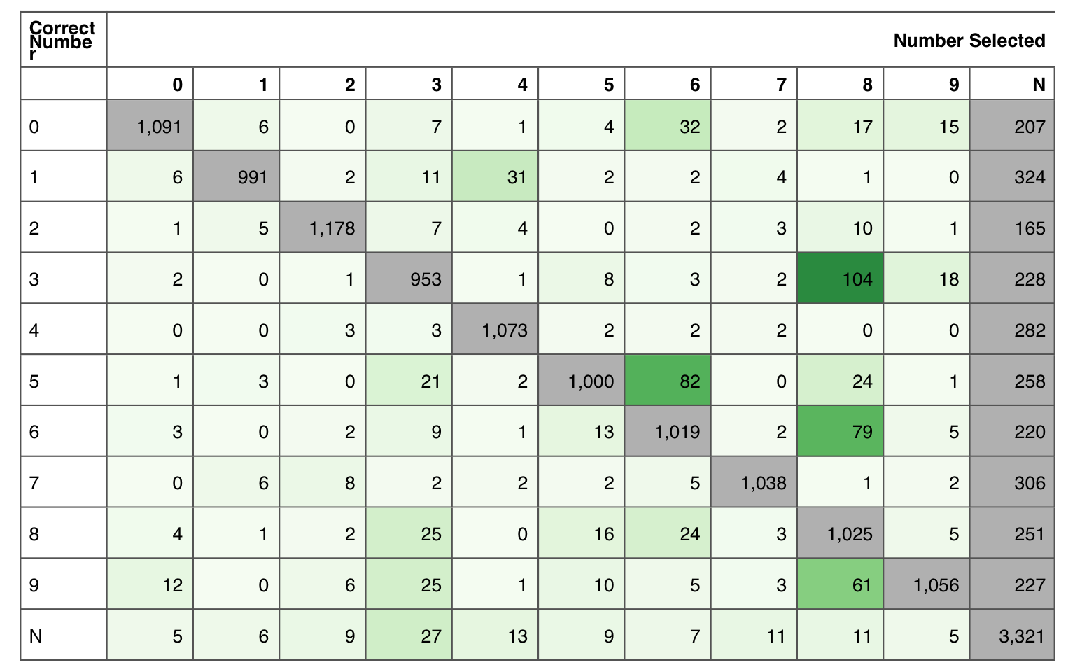
To understand the influence of the number displayed on the participant response, we can look at a confusion table of the number responses (Table 6.1).

Table 6.1: A confusion matrix of the number participants gave, alongside the true number in the plot. The off-diagonal elements are incorrect responses, with any concentration of numbers indicating values that are frequently mistaken for one another: 8 for 3, 6 and 9, and 6 for 5 are the most common.

For the cases where there actually was a number visible, we can see that participants typically got the number right, or selected no number visible, rather than making an incorrect guess. When there was no number, participants seemed to guess 3 more often than the other numbers.

There are also a few numbers that participants seemed to get confused more often than others. If we focus on the cases where 50 or more incorrect guesses were made, we can see that 3, 6 and 9 were frequently reported as an 8, and 5 was frequently reported as a 6. This makes sense as we could consider the dots that make up 3, 6, and 9 to be a subset of those covered by 8, with a similar relationship existing between 5 and 6. Interestingly, the converse is not true. That is, 8 was not mistaken for a 3, 6, or 9, and 6 was not mistaken for 5. This seems to suggest that, when participants could not make out the number with confidence, they seemed to have a tendency to add in structure that wasn’t there, rather than miss structure that was there.

Table 6.2: Numbers that were most commonly identified as ‘no number visible’, ordered from most to least frequent. The order roughly coincides, inversely, with the number of ‘dots’ that make up the number, suggesting that numbers constructed with fewer dots are harder to identify.

Selected	Correct	Total	Dots

No number visible	1	324	115
No number visible	7	306	150
No number visible	4	282	185
No number visible	5	258	215
No number visible	8	251	252
No number visible	3	228	211
No number visible	9	227	237
No number visible	6	220	226
No number visible	0	207	212
No number visible	2	165	228

Additionally, the number 1 (and possibly 7) were more frequently reported as no number visible relative to the other numbers (Table 6.2). This might be due to those numbers having less circles in the “number” group relative to the “background” group, as we can see the top 3 numbers reported as “no number” also had the lowest number of “number” dots relative to those in the background. However, this trend seems to drop off after 1, 7, and 4.

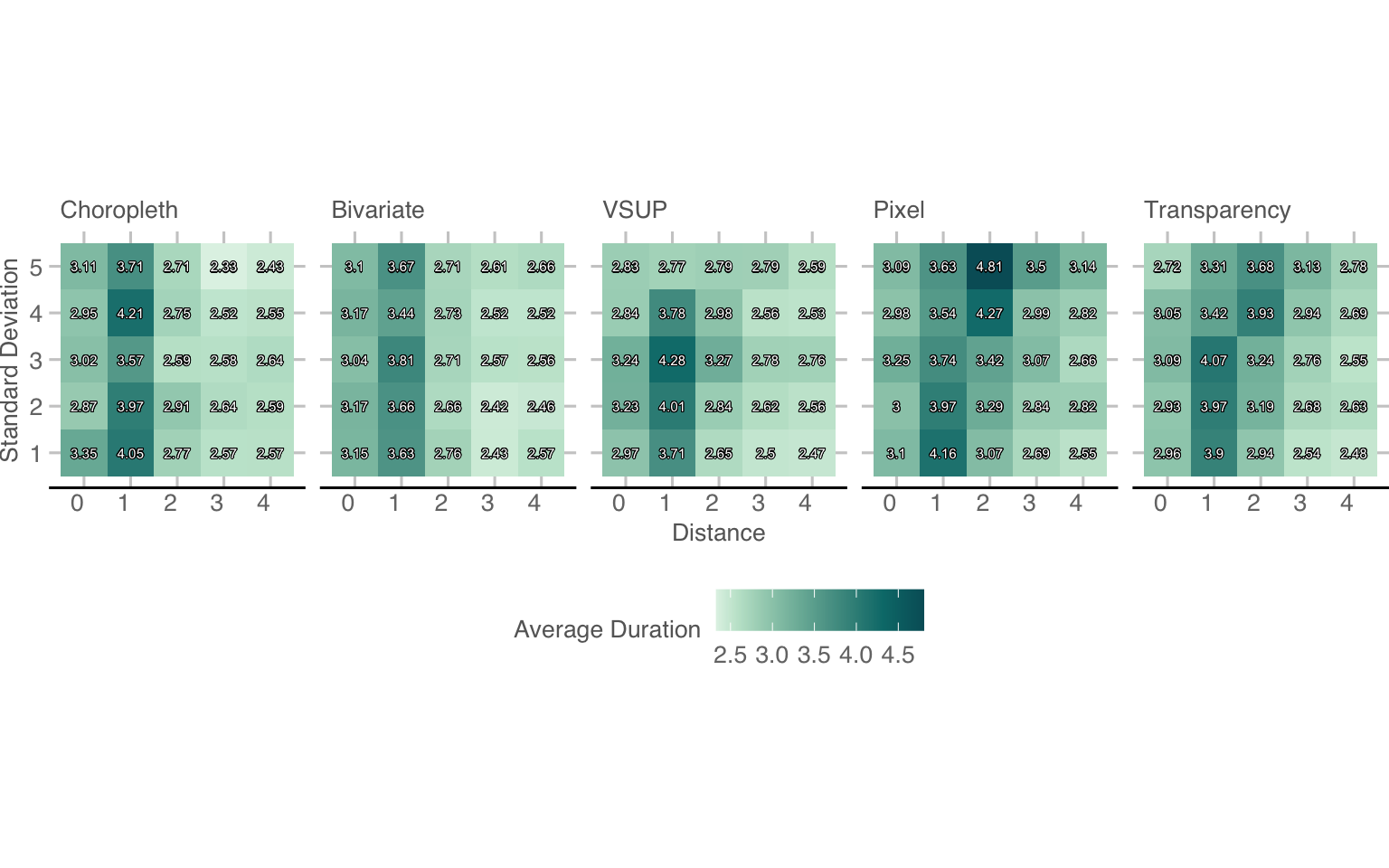
6.3 Duration Analysis

The trend in the amount of time participants spent on each question seems to align with the probability of getting the question correct. Figure 6.7 shows the median amount of seconds spent on each D, V, and plot type. Unsurprisingly, the most amount of time across all plots was on the D=1 case, when the signal was not particularly strong. The pixel and transparency maps have a lower triangle of easy to see numbers, that become harder to extract as both D decreases and V increases. It is also clear that participants rarely spent more than a few seconds on each plot. This also highlights that, by making uncertainty something that should be visibly seen, a well designed uncertainty visualisation can be correctly within a few seconds.

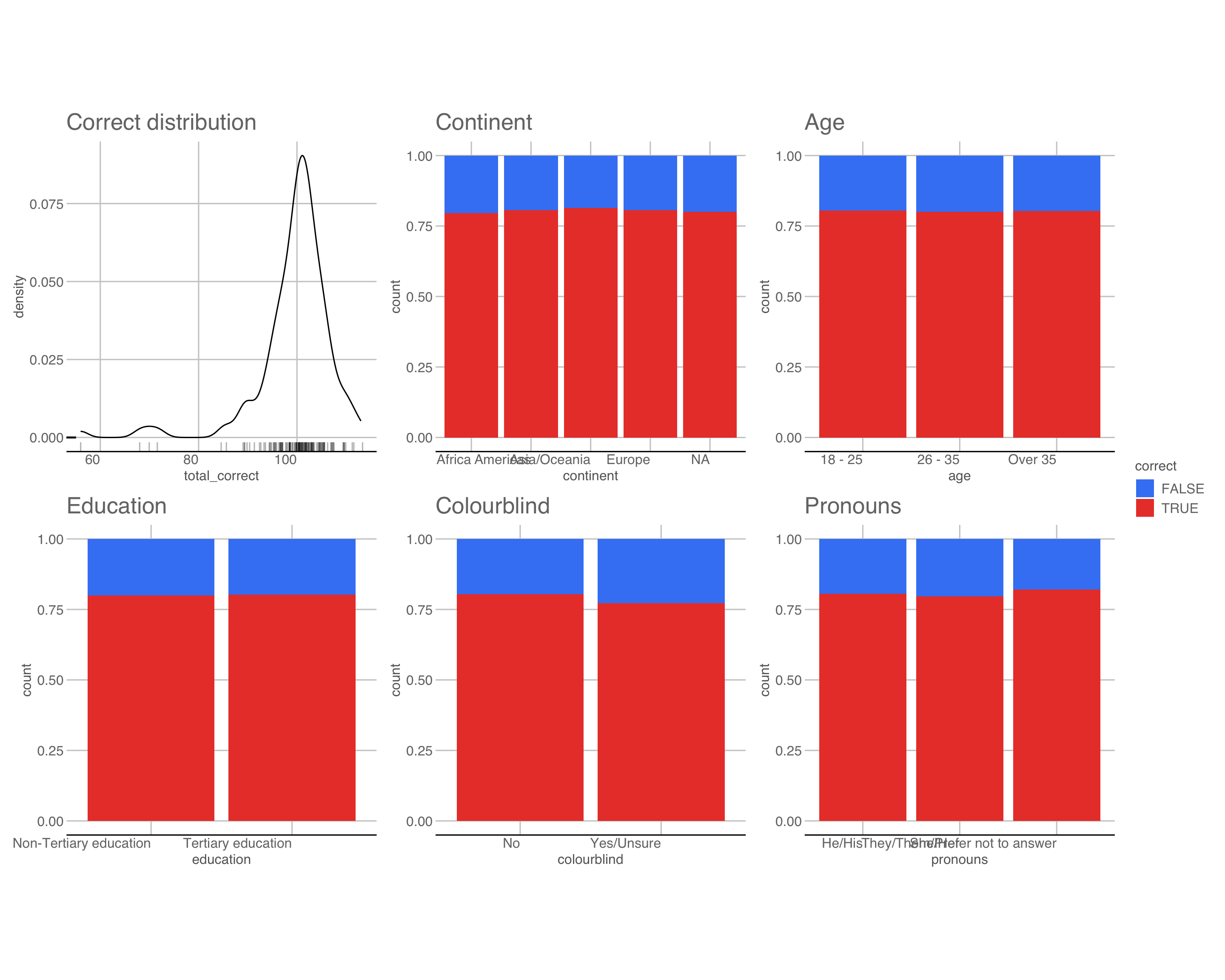
Figure 6.7: A heatmap showing the median duration accross each D, V, and plot type.

6.4 Demographic Analysis

The demographic analysis indicates no relationship between the demographic details and the proportion of correct responses.

Plots showing the overall distribution of correct answers from the participants, as well as the relationship betweeen the five demographic responses and the probability of correctly identifying the number in the stimuli.

6.5 Additional model comparison results

The distance-based results as well as all pairwise comparisons, as mentioned in the main text.

Table 6.3: Results for Standard Deviation Trend by Plot Type at Distance = 1

plot_type	V.trend	SE	z.ratio	p.value
Choropleth	-0.026	0.056	-0.460	0.646
Bivariate	-0.039	0.055	-0.701	0.484
VSUP	-0.577	0.059	-9.712	0.000
Pixel	-0.515	0.063	-8.234	0.000
Transparency	-0.538	0.066	-8.216	0.000

Table 6.4: Results for Standard Deviation Trend by Plot Type at Distance = 2

Table 6.5: Results for Standard Deviation Trend by Plot Type at Distance = 3

plot_type	V.trend	SE	z.ratio	p.value
Choropleth	0.245	0.190	1.288	0.198
Bivariate	-0.045	0.160	-0.278	0.781
VSUP	-3.121	0.139	-22.458	0.000
Pixel	-0.762	0.077	-9.870	0.000
Transparency	-0.624	0.092	-6.753	0.000

Table 6.6: Results for Standard Deviation Trend by Plot Type at Distance = 4

plot_type	V.trend	SE	z.ratio	p.value
Choropleth	0.381	0.290	1.316	0.188
Bivariate	-0.047	0.245	-0.193	0.847
VSUP	-4.394	0.209	-21.040	0.000
Pixel	-0.886	0.124	-7.154	0.000
Transparency	-0.667	0.149	-4.475	0.000

Table 6.7: Results for Standard Deviation Trend by Plot Type at Distance = 1

contrast	estimate	SE	z.ratio	p.value
Choropleth - Bivariate	0.013	0.078	0.166	1.000
Choropleth - VSUP	0.551	0.081	6.763	0.000
Choropleth - Pixel	0.490	0.084	5.847	0.000
Choropleth - Transparency	0.513	0.086	5.965	0.000
Bivariate - VSUP	0.538	0.081	6.639	0.000
Bivariate - Pixel	0.476	0.083	5.715	0.000
Bivariate - Transparency	0.500	0.086	5.835	0.000
VSUP - Pixel	-0.062	0.086	-0.716	0.953
VSUP - Transparency	-0.038	0.088	-0.435	0.993
Pixel - Transparency	0.023	0.090	0.257	0.999

Table 6.8: Results for Standard Deviation Trend by Plot Type at Distance = 2

contrast	estimate	SE	z.ratio	p.value
Choropleth - Bivariate	0.153	0.128	1.190	0.757
Choropleth - VSUP	1.960	0.125	15.674	0.000
Choropleth - Pixel	0.749	0.109	6.897	0.000
Choropleth - Transparency	0.693	0.111	6.265	0.000
Bivariate - VSUP	1.807	0.113	15.974	0.000
Bivariate - Pixel	0.596	0.095	6.289	0.000
Bivariate - Transparency	0.540	0.097	5.563	0.000
VSUP - Pixel	-1.211	0.090	-13.515	0.000
VSUP - Transparency	-1.267	0.092	-13.766	0.000
Pixel - Transparency	-0.056	0.069	-0.821	0.924

Table 6.9: Results for Standard Deviation Trend by Plot Type at Distance = 3

contrast	estimate	SE	z.ratio	p.value
Choropleth - Bivariate	0.292	0.253	1.157	0.776
Choropleth - VSUP	3.369	0.238	14.130	0.000
Choropleth - Pixel	1.009	0.208	4.843	0.000
Choropleth - Transparency	0.873	0.215	4.068	0.000
Bivariate - VSUP	3.076	0.214	14.361	0.000
Bivariate - Pixel	0.716	0.180	3.972	0.001
Bivariate - Transparency	0.580	0.188	3.094	0.017
VSUP - Pixel	-2.360	0.159	-14.864	0.000
VSUP - Transparency	-2.496	0.167	-14.939	0.000
Pixel - Transparency	-0.136	0.121	-1.124	0.794

Table 6.10: Results for Standard Deviation Trend by Plot Type at Distance = 4

contrast	estimate	SE	z.ratio	p.value
Choropleth - Bivariate	0.432	0.385	1.122	0.795
Choropleth - VSUP	4.778	0.361	13.238	0.000
Choropleth - Pixel	1.268	0.319	3.975	0.001
Choropleth - Transparency	1.052	0.330	3.191	0.012
Bivariate - VSUP	4.346	0.325	13.357	0.000
Bivariate - Pixel	0.836	0.278	3.003	0.022
Bivariate - Transparency	0.620	0.291	2.133	0.206
VSUP - Pixel	-3.509	0.243	-14.453	0.000
VSUP - Transparency	-3.725	0.257	-14.486	0.000
Pixel - Transparency	-0.216	0.195	-1.107	0.803